Category: Observability

Guides to metrics, logs and traces in production: OpenTelemetry, SLOs, high-cardinality costs and keeping monitoring bills under control.

  • SLOs for Small Teams: Error Budgets Without an SRE Department

    SLOs for Small Teams: Error Budgets Without an SRE Department

    SLOs for small teams have a reputation problem: they look like something only Google can afford to run. They aren’t.

    Ask most teams what their reliability target is and you get “99.9% uptime.” Ask what that measures, and the conversation gets vague. Uptime of what? Measured from where? Does a page that loads in twelve seconds count as up?

    That vagueness is why the number never changes any decision. A reliability target that doesn’t tell you what to work on next week isn’t a target, it’s a slogan.

    Service Level Objectives fix this, and the usual objection is that SLOs are a Google thing requiring a dedicated SRE organisation. They aren’t. A four-person team can run meaningful SLOs on two metrics per service. Here’s how small teams can set SLOs, spend an error budget and alert on burn rate, without the ceremony.

    The three terms, quickly

    SLI — Service Level Indicator. A measurement. “The proportion of HTTP requests that returned a non-5xx status.” A number between 0 and 1.

    SLO — Service Level Objective. A target for that measurement over a window. “99.9% of requests return non-5xx, measured over 28 days.” Internal. You choose it.

    SLA — Service Level Agreement. A contractual promise to a customer, with financial consequences. Set it looser than your SLO, always. Your SLO is the line where you start worrying; your SLA is the line where you start refunding. If they’re the same number, you find out about problems from your customers’ lawyers.

    The one that does the work is the SLO.
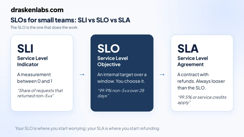
    SLOs for small teams: how an SLI, an SLO and an SLA differ
    How SLOs relate to SLIs and SLAs.

    The error budget is the whole point

    If your SLO is 99.9% over 28 days, you are explicitly saying that 0.1% failure is acceptable. That 0.1% is your error budget, and turning it into time makes it concrete:

    SLODowntime per 28 daysPer year
    99%6h 43m3d 15h
    99.5%3h 22m1d 19h
    99.9%40m 19s8h 45m
    99.95%20m 10s4h 23m
    99.99%4m 2s52m

    Look at 99.99% for a moment. Four minutes a month. That is less time than it takes a human to read a page, open a laptop, and log in. Hitting four nines means automated failover with no human in the loop, multi-region redundancy, and deployment practices that make bad releases nearly impossible. It is a different engineering budget entirely, not a slightly better version of three nines.

    This is the first thing an error budget does for you: it makes reliability targets cost something, so they stop being chosen by whoever wants to sound most ambitious in the meeting.

    The second thing is that it reframes reliability work as a resource rather than a virtue. You have not “failed” if you consumed 60% of your budget. You have used a resource you were allocated, buying deployment velocity with it. Budget remaining means ship faster. Budget exhausted means stop and fix. That’s a decision rule, which is more than “we value reliability” ever gave you.
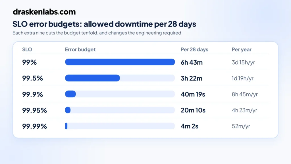
    SLOs and error budgets: allowed downtime per 28 days for 99% to 99.99% targets
    Error budgets for common SLOs over a 28-day window.

    Choosing SLIs that mean something

    Two rules cover most of it.

    Measure what the user experiences, not what the server reports. CPU utilisation is not an SLI. Neither is memory, disk, or pod restart count. Those are diagnostics — useful once something is wrong, useless as a definition of “wrong.” A service can be at 95% CPU and perfectly healthy, or at 5% CPU and completely broken.

    Never use averages for latency. Average response time is the single most misleading metric in production. If 95% of requests take 50ms and 5% take 30 seconds, your average looks acceptable and one in twenty of your users is furious. Use a threshold instead: the proportion of requests completing under 500ms. Now it’s a ratio, it composes with your availability SLI, and it can’t hide a tail.

    For most request-serving services, two SLIs is the right number:

    • Availability: successful requests ÷ valid requests
    • Latency: requests under threshold ÷ valid requests

    “Valid requests” matters. Exclude 4xx client errors from availability — a user sending a malformed request is not your service failing. Exclude health checks and synthetic traffic, or you’ll dilute your own signal with things no user ever touches.

    For non-request workloads, adapt the shape rather than the concept. Data pipelines: freshness, “the proportion of hours where output was less than 15 minutes stale.” Queue consumers: “the proportion of messages processed within 30 seconds of enqueue.” Batch jobs: completion within the expected window.

    Setting the target: measure first, then decide

    The most common failure is picking a target aspirationally. Someone says 99.9%, everyone nods, and three weeks later you’re missing it constantly, alerts are firing, and the team has learned to ignore them.

    Do it the other way round. Instrument the SLI, collect four weeks of data, and look at what you actually deliver. If you’re currently at 99.5%, set the SLO at 99.5%. Not 99.9%.

    That feels like cheating. It isn’t. The job of SLOs is to tell you when something has changed for the worse. A target you meet 99% of the time does that. A target you miss constantly tells you nothing except that you set it badly, and it trains your team to ignore the signal — which is a genuinely expensive thing to teach people.

    Once you’re comfortably meeting it, tighten it. Reliability targets should ratchet.

    The other half of the question is what your users actually need. A B2B tool used during Indian business hours has a different profile than a payments API. If your customers barely notice a two-minute blip, three nines may be more than they’re paying for, and the engineering effort is better spent elsewhere. Reliability beyond what users perceive is money you have set on fire.

    Burn rate alerting, not threshold alerting

    This is where SLOs stop being documentation and start improving your on-call.

    The naive approach is to alert when one of your SLOs is breached. Too late — you’ve already spent the budget. The slightly-less-naive approach is to alert on any error rate above zero, which pages you at 3am for a blip that consumed four seconds of a forty-minute budget.

    Burn rate solves this. Burn rate is how fast you’re consuming the error budget relative to the rate that would exhaust it exactly at the end of the window. Burn rate 1 means you’ll finish the month right on target. Burn rate 14.4 means you’ll exhaust a 28-day budget in about two days.

    The standard pattern, from the Google SRE workbook, uses two alerts:

    • Fast burn: burn rate above 14.4 sustained over 1 hour → page someone. Something is badly broken right now.
    • Slow burn: burn rate above 6 sustained over 6 hours → raise a ticket, don’t page. Something is degrading steadily and needs attention this week, not tonight.

    Each alert uses two windows — a long one for signal and a short one to confirm the problem is still happening — so alerts resolve when the incident does rather than lingering.

    The practical effect is that your pager fires on user-visible harm, proportional to severity. A brief spike that costs you thirty seconds of budget doesn’t wake anyone. A sustained failure does, immediately. Most teams we work with cut their page volume by more than half in the first month after switching, which does more for reliability than any dashboard, because a team that trusts its pager investigates instead of dismissing.
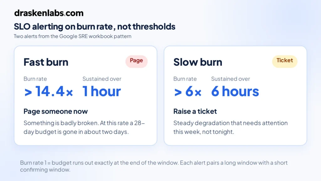
    SLO burn-rate alerting: fast burn above 14.4x over 1 hour pages, slow burn above 6x over 6 hours raises a ticket
    Burn-rate alerting for SLOs: fast burn pages someone, slow burn raises a ticket.

    The error budget policy

    An error budget without an agreed consequence is a chart nobody looks at. Write down, before you need it, what happens at each threshold. One page is enough:

    • Budget above 50% remaining: normal operation. Ship features.
    • Below 25%: no risky deployments. No schema migrations on Friday. Reliability items get pulled into the sprint.
    • Exhausted: feature work pauses. The team works on reliability until the budget recovers.
    • Two consecutive windows exhausted: the SLO was wrong or the architecture is inadequate. Escalate to a design conversation, not more heroics.

    The value here is that it’s agreed in advance, in calm conditions. Arguing about whether to pause the roadmap during an outage is a bad time to first discover that engineering and product have different views.

    Get explicit sign-off from whoever owns the roadmap. An error budget policy that engineering wrote alone is a policy that gets overruled the first time it’s inconvenient.
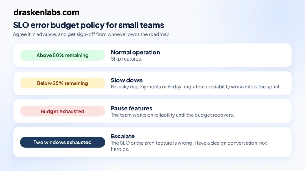
    SLO error budget policy thresholds: normal operation, slow down, pause features, escalate
    An error budget policy agreed before SLOs are breached.

    Where teams go wrong

    Too many SLOs. Every service, four indicators each, thirty dashboards nobody reads. Start with your two or three most important user-facing services and one or two SLIs each. That is enough to change behaviour, which is the only test that matters.

    SLOs on internal services. If a user never touches it directly, its reliability matters only through its effect on something they do touch. Measure the user-facing thing. Internal service health is a diagnostic.

    A 100% target. Not achievable, and it destroys the mechanism. Zero error budget means every deploy is a violation, so the concept gets abandoned within a month.

    Never revisiting them. Traffic patterns change, architectures change, user expectations change. Review targets quarterly.

    Tracking without acting. The most common outcome by far. A beautiful Grafana dashboard, burn-rate alerts wired up, and no agreed consequence when the budget goes. It becomes decoration. The policy is not the boring part of SLOs, it’s the entire point.

    Making SLOs work for small teams in practice

    You don’t need a platform team. On a Prometheus and Grafana stack: recording rules to compute the SLI ratios, multi-window burn-rate alerts in Alertmanager, one Grafana panel per SLO showing budget remaining. Sloth generates the rules from a short YAML spec if you’d rather not hand-write them, and OpenSLO gives you a vendor-neutral format if you expect to move backends. Datadog, Grafana Cloud, and Honeycomb all have native support for SLOs if you’re already paying for one.

    The instrumentation matters more than the tooling. Your SLIs are only as good as the data underneath them, which is a question of how you’ve instrumented your services and how much of that data you can afford to keep — the cardinality problem that quietly determines what your observability stack costs.

    We took one healthtech client from no coverage across 200+ microservices to full instrumentation with SLOs and burn-rate alerting in under two weeks, cutting mean time to detect below two minutes. The instrumentation was the fast part. Agreeing what “good” meant for each service took longer, and mattered more.

    If your alerts fire constantly and nobody trusts them, that’s usually an SLO problem wearing a monitoring costume. Tell us what you’re running and we’ll take a look — it’s the core of our observability work.

    Sources and further reading

  • High Cardinality Metrics: Why Your Observability Bill Grew 4x

    High Cardinality Metrics: Why Your Observability Bill Grew 4x

    High cardinality metrics are the reason, almost every time.

    Traffic grew 30% this year. The observability bill grew 400%. Nobody changed the vendor, nobody added a new tool, and no single person can explain what happened.

    This is one of the most common infrastructure cost surprises we see, and it’s almost always the same cause. Observability platforms do not bill by traffic. They bill by the number of distinct things you ask them to remember. That number is cardinality, and it multiplies rather than adds.

    Once you understand the multiplication, the fix is mechanical.

    What high cardinality metrics actually are

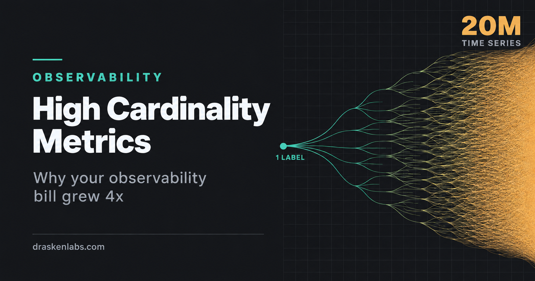
    A metric is not one number. A metric with labels is one number per unique combination of label values, and each of those combinations is a separate time series that has to be stored, indexed, and queried.

    Take a request counter:

    http_requests_total{service, endpoint, method, status}

    With 10 services, 20 endpoints, 4 methods, and 5 status codes, that’s 10 × 20 × 4 × 5 = 4,000 time series. Entirely fine.

    Now someone adds customer_id to help debug a support ticket. You have 5,000 customers.

    4,000 × 5,000 = 20 million time series, from one line of code.

    The traffic didn’t change. The number of requests didn’t change. But your storage, your index size, your query latency, and your bill all changed by three orders of magnitude, and the commit that did it looked completely reasonable in review.

    This is the shape of nearly every observability cost incident: a small, sensible-looking change to a label set.

    The labels that cause it

    Some values are unbounded by nature. Putting any of these in a metric label is how you get the 400% bill.

    • User or customer identifiers. Grows with your business. This is the classic.
    • Request or trace IDs. Unique per request. Every single request creates a new time series that is written once and never queried again.
    • Raw URL paths. /api/users/8f3a2b and /api/users/c91e4d are different label values. Every user ID in a path becomes a series.
    • Email addresses, session tokens, order numbers. Same problem, and often a privacy issue on top.
    • Container, pod, or instance IDs. Subtler and very common. In a Kubernetes environment with rolling deploys, pod names change on every release. Deploy ten times a day and you generate ten new sets of series daily, most of them dead within the hour but still stored, still indexed, still billed.
    • Full error messages. "connection refused to 10.0.4.19:5432" is not a label value. "connection_refused" is.
    • Timestamps. Rare but catastrophic. Every scrape becomes a new series.

    The pod-ID one deserves emphasis because it hides. Nobody deliberately adds it — it arrives by default from a Kubernetes service discovery config or an auto-instrumentation library, and it silently multiplies your entire metric set by your deploy frequency.

    The rule that resolves it

    Metrics, traces, and logs have different cost profiles, and the discipline is to put each dimension where it belongs.

    Metrics are for low-cardinality aggregate questions. How many requests, how many errors, what’s the p99. Bounded labels only: service name, endpoint template, method, status class, environment, region. If a label’s value set could grow without limit, it does not belong on a metric.

    Traces are for high-cardinality specifics. This is the correct home for user IDs, request IDs, order numbers, feature flag states, and full URLs. Span attributes are stored per-span, not as a cross-product, so adding an attribute costs you linearly rather than multiplicatively. The rule of thumb: anything you want to filter one request by belongs on a span; anything you want to graph over time belongs on a metric.

    Logs are for detail, sampled and retained deliberately. Cheap per event, ruinous in aggregate. CloudWatch Logs bills around $0.50 per GB ingested; most vendors are comparable. A service logging every health check at debug level generates a remarkable amount of money’s worth of nothing.

    Almost every cardinality problem we’ve debugged was a high-cardinality dimension that had been put on a metric when it should have been on a span.

    Templating your paths

    The single highest-value fix, and the one most often missed.

    Auto-instrumentation frequently records the raw request path. You want the route template:

    BAD:   http_requests_total{path="/api/users/8f3a2b/orders/119"}
    GOOD:  http_requests_total{route="/api/users/{id}/orders/{order_id}"}

    Most frameworks expose the matched route rather than the raw path — Express, FastAPI, Spring, Rails all do. Use it. The OpenTelemetry semantic conventions specify http.route for exactly this reason, and if your instrumentation is populating http.target into a metric label instead, that’s your bug.

    While you’re there: use the semantic conventions generally. Naming your attributes http.request.method and service.name rather than inventing your own means your dashboards and alerts survive a change of vendor or instrumentation library, which is worth more than it sounds like the day you need it.

    The Collector is your control point

    Instrumenting every service to emit exactly the right data, and keeping it that way as forty developers commit, is not achievable. Put the enforcement somewhere central instead.

    The OpenTelemetry Collector sits between your applications and your backend. Everything passes through it, which makes it the one place you can apply policy without touching application code.

    Drop attributes before they reach the backend. An attributes processor can delete user.id and session.token from metrics while leaving them on spans. One config change, applied to every service.

    Filter what you don’t need. Health check spans, /metrics scrapes, readiness probes. These are pure noise and they’re often a double-digit percentage of your span volume.

    Batch. Reduces network overhead and, with per-request-billing vendors, directly reduces cost.

    Switch backends without redeploying anything. Because your applications speak OTLP to the Collector and only the Collector knows about your vendor, changing vendors is a config change. This is the strongest practical argument for OpenTelemetry over vendor-specific agents, and it’s worth setting up before you need it, not during a contract renegotiation.

    Run it as a DaemonSet for node-local collection, plus a gateway deployment for anything requiring a full view of a trace. That second part matters for the next section.

    Sampling traces properly

    You cannot afford to store every trace at any real volume. The question is which ones you keep.

    Head sampling decides at the start of the request, usually with a fixed probability. Cheap, simple, and stateless — but it decides before knowing whether the request failed or took nine seconds. At 1% head sampling you throw away 99% of your errors, which are the traces you actually wanted.

    Tail sampling buffers complete traces and decides after seeing the outcome. This is what you want:

    • Keep 100% of traces containing an error
    • Keep 100% of traces above a latency threshold
    • Keep 100% of traces for low-traffic endpoints, which would otherwise vanish entirely
    • Keep 1–5% of everything else as a healthy baseline

    The result is that you store a small fraction of your volume while retaining essentially all of the diagnostically interesting traces. Ten to twenty times cost reduction with better debugging is not a typical trade in infrastructure, and it’s available here.

    The catch: tail sampling requires all spans of a trace to reach the same Collector instance. That means a gateway tier with trace-ID-aware load balancing in front of it, and memory sized for your buffering window. It’s a real piece of architecture, not a config flag, but it’s a day’s work and it pays for itself immediately.

    Log discipline

    Three changes cover most of the waste.

    Drop noise at the source. Health checks, readiness probes, and load balancer pings should be filtered at the agent or Collector, not ingested and then ignored. This is frequently 20–40% of log volume in a Kubernetes environment.

    Structure your logs. JSON, with consistent field names, and the trace ID included so you can jump from a log line to the full trace. Unstructured logs force you to pay for full-text indexing to get anything back out.

    Tier your retention. Seven days hot and searchable, ninety days in object storage for compliance, nothing beyond that unless a regulator says otherwise. Setting explicit retention on every log group matters because the default on most platforms is “keep forever,” which is almost never what anyone intended.

    And the recurring one: audit your log levels in production. Debug logging left on after an incident is one of the most common causes of a sudden bill increase we see.

    A quick audit

    Half a day, and it usually finds most of it.

    1. Find your top series by cardinality. On Prometheus, topk(20, count by (__name__)({__name__=~".+"})) shows which metric names generate the most series. On Datadog, the custom metrics breakdown does the same. The offender is usually obvious and usually a single metric.
    2. Check your top ten metrics’ label sets. Any label whose value set could grow unboundedly is a finding.
    3. Grep for raw paths. Search dashboards and metric names for anything containing a UUID or a numeric ID.
    4. Measure health check traffic. As a proportion of total spans and log lines. If it’s over 10%, filter it today.
    5. Confirm your sampling strategy. If you’re head sampling at a low rate, you’re discarding errors. Move to tail sampling.
    6. List log groups with no retention policy. Set one on all of them.

    The point isn’t just the bill

    Cost is the visible symptom. The real damage from cardinality explosion is that queries slow down, dashboards time out, and your team stops using the observability stack during incidents because it’s too slow to be useful mid-outage. Cardinality discipline is a reliability practice that happens to also save money.

    There’s a connection to targets here too. Your SLOs are computed from metrics, so a metric set that’s too expensive to query at speed is a burn-rate alert that fires late. And the same cost-attribution discipline that works on cloud infrastructure spend applies to telemetry: without knowing which service generates which cost, nobody owns reducing it.

    If your observability bill has outgrown its usefulness, that’s the kind of thing our observability engagements start with. Send us the shape of your setup and we’ll tell you where it’s going.

    What is high cardinality in metrics?

    Cardinality is the number of unique time series a metric produces, calculated as the product of all its label value counts. High cardinality means that product is large, usually because a label like user ID or request ID has an unbounded set of values. Cost and query latency scale with it.

    Why did my Datadog or Prometheus bill increase without more traffic?

    Almost always a new label with many possible values added to an existing metric, or auto-instrumentation recording raw URL paths instead of route templates. Both multiply your series count without changing request volume. Check which metric names produce the most series first.

    Where should user IDs go if not in metric labels?

    On span attributes. Traces store attributes per span rather than as a cross-product, so a user ID adds cost linearly rather than multiplicatively, and traces are the right tool for investigating individual requests anyway.

    What is tail sampling and why is it better than head sampling?

    Tail sampling decides whether to keep a trace after seeing the complete result, so you can retain all errors and slow requests while discarding most successful ones. Head sampling decides at the start and therefore discards errors at the same rate as everything else.

    How much can we realistically cut observability costs?

    Teams that have never audited cardinality typically find 40–70%, mostly from dropping unbounded labels, filtering health checks, and moving to tail sampling. Query performance usually improves at the same time.

    Does OpenTelemetry lock us into a vendor?

    No, and that’s largely the point. Applications emit OTLP to a Collector, and only the Collector is configured with your backend. Switching vendors is a Collector config change rather than a re-instrumentation project.